Notebook. Demographics
# Work from this notebook's folder (content/), also when the notebook is executed from the project root
# (myst build --execute, NeuroLibre), so the local modules (helpers, stats_test, ...) and ../data/ resolve.
import os
import sys

if os.path.isdir("content") and not os.path.isfile("helpers.py"):
    os.chdir("content")
if os.getcwd() not in sys.path:
    sys.path.insert(0, os.getcwd())
import pandas as pd
import numpy as np
import seaborn as sns
import matplotlib.pyplot as plt
from tableone import TableOne
import helpers
import plotly.express as pxtsv = helpers.data_path("participants.tsv")
df= pd.read_csv(tsv, sep='\t').convert_dtypes()# Define the desired order of categories
group_order = ['HC', 'LBD', 'FTD', 'AD']
# Convert to ordered categorical type (the data files code healthy controls as 'Control'; the paper uses HC)
df['group'] = df['group'].replace({'Control': 'HC'})
df['group'] = pd.Categorical(df['group'], categories=group_order, ordered=True)Demographics
# Set style
sns.set_theme(style="whitegrid")

# Create subplots
fig, axes = plt.subplots(1, 3, figsize=(15,5))

# 1. Age distribution
sns.histplot(df['age'], kde=True, ax=axes[0], color="skyblue")
axes[0].set_title("Age Distribution")

# 2. Sex counts
sns.countplot(x="sex", data=df, ax=axes[1], hue="sex", palette="pastel")
axes[1].set_title("Sex Distribution")

# 3. Group counts
sns.countplot(x="group", data=df, ax=axes[2], hue="group", palette="muted")

axes[2].set_title("Group Distribution")

# Adjust layout
plt.tight_layout()
plt.show()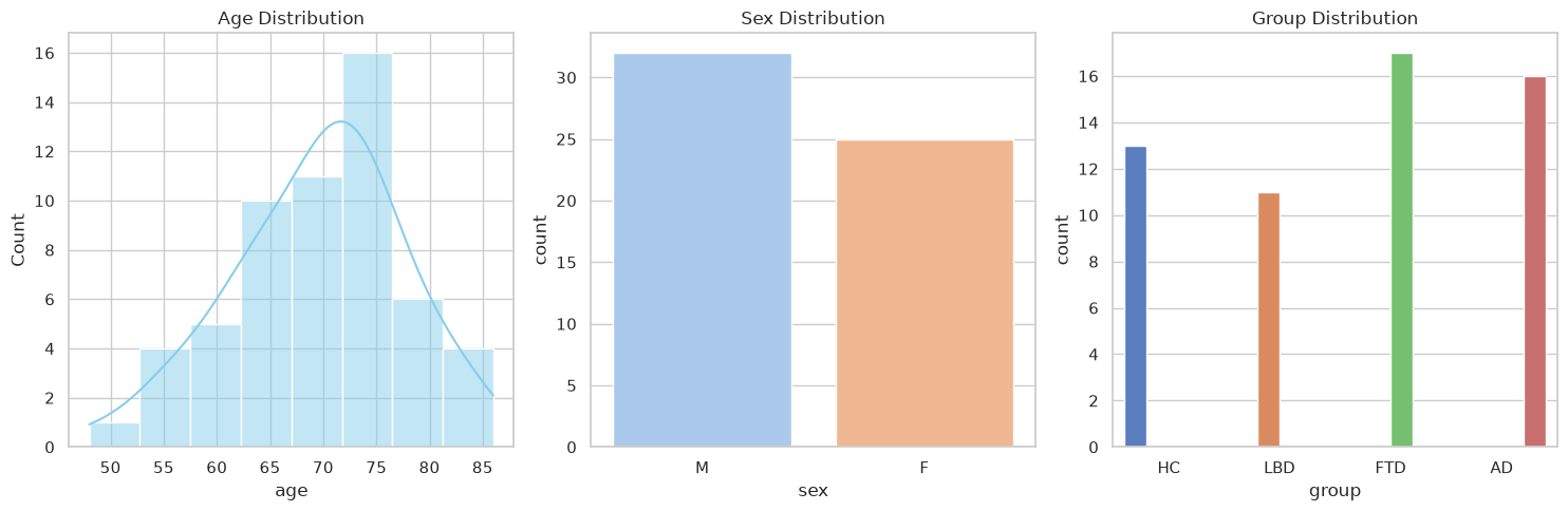
Total subjects:
len(df)57Total subject per group:
print(df["group"].value_counts())group
FTD 17
AD 16
HC 13
LBD 11
Name: count, dtype: int64
Demographics table:
columns = ["age", "sex", "MoCA"]
categorical = ["sex"]

#mean (SD) shown for all continuous vars, ANOVA/chi-square used for p-values.
table_demographics = TableOne(
    df,
    columns=columns,
    categorical=categorical,
    groupby="group",
    pval=True,
    htest_name=True
)

# Get Pandas dataframe
table_demographics = table_demographics.tableone.copy()

# Flatten the "Grouped by group" column header down to just the group names,
# and drop the "Missing" column (always 0 here, so it adds nothing).
table_demographics.columns = table_demographics.columns.get_level_values(1)
table_demographics = table_demographics.drop(columns="Missing")

# Role per row, in the same order as table before
table_demographics.insert(0, "Role", [
    "",                   # n
    "Covariate",          # age, mean (SD)
    "Covariate",          # sex, n (%) -- F
    "Covariate",          # sex, n (%) -- M
    "Descriptive only",   # MoCA, mean (SD)
    #"Descriptive only",   # years_diagnosis, mean (SD)
])

# remove warnings from table. An alternative approach was used to validate the results.
table_demographics["Test"] = table_demographics["Test"].str.replace(
    r"Chi-squared \(warning: expected count < 5\)", "Chi-squared", regex=True)

helpers.display_table(table_demographics.reset_index().rename(columns={'level_0': 'Characteristic', 'level_1': ''}))
Loading...
# Build histogram
fig = px.histogram(
    df,
    x="age",
    color="group",
    pattern_shape="sex",   # distinguishes male/female inside groups
    barmode="stack",       # stack sex inside group
    opacity=0.8,
    nbins=10,
    color_discrete_map={
    "AD": "red",
    "LBD": "orange",
    "FTD": "green",
    "HC": "blue"
    },
    width=750,
    height=500
)

# Improve layout
fig.update_layout(
    title="Age Distribution by Group and Sex",
    xaxis_title="Age",
    yaxis_title="Count",
    bargap=0.05,
    legend_title="Group / Sex"
)

fig.show()
Loading...
Removing Subject with failed segmentation
# Exclusion list obtained from QC the segemntation and registration of the anatomical scans. Participants with a QC level of 0 were excluded from the analyses.
exclusion_list = pd.read_csv(helpers.data_path("exclusion_list.csv"))
print(exclusion_list)
exclusion_list = exclusion_list["participant_id"].to_list()
participant_id reason
0 sub-021 HippUnfold segmentation with a small leak arti...
1 sub-024 HippUnfold segmentation slightly failed: SRLM ...
2 sub-035 HippUnfold segmentation failed with an artifac...
3 sub-045 HippUnfold segmentation slightly failed with s...
4 sub-049 HippUnfold segmentation failed with subiculum ...
5 sub-051 HippUnfold segmentation struggled with multipl...
6 sub-057 HippUnfold segmentation failed with small leak...
df_removed = df.query("participant_id == @exclusion_list")
df = df.query("participant_id != @exclusion_list")
print("Subjects exclude because failed segmentation (QC = 0):")
print(df_removed["group"].value_counts())Subjects exclude because failed segmentation (QC = 0):
group
FTD 4
AD 2
LBD 1
HC 0
Name: count, dtype: int64
# Set style
sns.set_theme(style="whitegrid")

# Create subplots
fig, axes = plt.subplots(1, 3, figsize=(15,5))

# 1. Age distribution
sns.histplot(df['age'], kde=True, ax=axes[0], color="skyblue")
axes[0].set_title("Age Distribution")

# 2. Sex counts
sns.countplot(x="sex", data=df, ax=axes[1], hue="sex", palette="pastel")
axes[1].set_title("Sex Distribution")

# 3. Group counts
sns.countplot(x="group", data=df, ax=axes[2], hue="group", palette="muted")

axes[2].set_title("Group Distribution")

# Adjust layout
plt.tight_layout()
plt.show()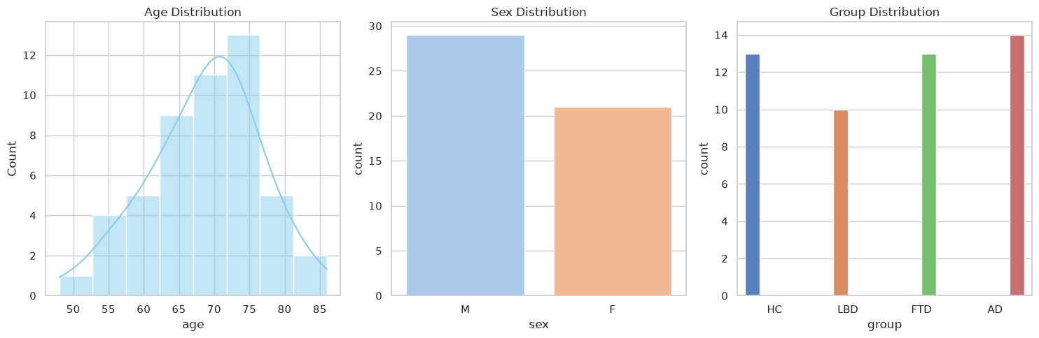
# Total subject in the study after failed segementation removal
len(df)50# Total subject in each group after failed segementation removal
print(df["group"].value_counts())group
AD 14
HC 13
FTD 13
LBD 10
Name: count, dtype: int64
columns = ["age", "sex", "MoCA"]
categorical = ["sex"]

#mean (SD) shown for all continuous vars, ANOVA/chi-square used for p-values.
table_demographics = TableOne(
    df,
    columns=columns,
    categorical=categorical,
    groupby="group",
    pval=True,
    htest_name=True
)

# Get Pandas dataframe
table_demographics = table_demographics.tableone.copy()

# Flatten the "Grouped by group" column header down to just the group names,
# and drop the "Missing" column (always 0 here, so it adds nothing).
table_demographics.columns = table_demographics.columns.get_level_values(1)
table_demographics = table_demographics.drop(columns="Missing")

# Role per row, in the same order as table before
table_demographics.insert(0, "Role", [
    "",                   # n
    "Covariate",          # age, mean (SD)
    "Covariate",          # sex, n (%) -- F
    "Covariate",          # sex, n (%) -- M
    "Descriptive only",   # MoCA, mean (SD)
    #"Descriptive only",   # years_diagnosis, mean (SD)
])

# remove warnings from test table. An alternative approach was used to validate the results.
table_demographics["Test"] = table_demographics["Test"].str.replace(
    r"Chi-squared \(warning: expected count < 5\)", "Chi-squared", regex=True)

helpers.display_table(table_demographics.reset_index().rename(columns={'level_0': 'Characteristic', 'level_1': ''}))
Loading...
# Build histogram
fig = px.histogram(
    df,
    x="age",
    color="group",
    pattern_shape="sex",   # distinguishes male/female inside groups
    barmode="stack",       # stack sex inside group
    opacity=0.8,
    nbins=10,
    color_discrete_map={
    "AD": "red",
    "LBD": "orange",
    "FTD": "green",
    "HC": "blue"
    },
    width=750,
    height=500
)

# Improve layout
fig.update_layout(
    title="Age Distribution by Group and Sex",
    xaxis_title="Age",
    yaxis_title="Count",
    bargap=0.05,
    legend_title="Group / Sex"
)

fig.show()
Loading...
# Static version of the demographics figure (analysed sample), used in the Word/PDF/LaTeX exports.
# Same design as the interactive figure: age histogram stacked by group, hatched bars for male participants
if helpers.STATIC_FIGURE_FORMATS:
    from matplotlib.patches import Patch

    helpers.static_theme()
    group_colors = dict(zip(group_order, sns.color_palette("deep")))
    bins = np.histogram_bin_edges(df["age"], bins=10)
    fig, ax = plt.subplots(figsize=(helpers.TEXT_WIDTH_IN / 2, 2.4))
    bottom = np.zeros(len(bins) - 1)
    for group in group_order:
        for sex, hatch in (("F", None), ("M", "////")):
            counts, _ = np.histogram(df.query("group == @group and sex == @sex")["age"], bins=bins)
            ax.bar(bins[:-1], counts, width=np.diff(bins), bottom=bottom, align="edge", color=group_colors[group],
                   hatch=hatch, edgecolor="white", linewidth=0.5)
            bottom += counts
    handles = ([Patch(facecolor=group_colors[g], label=g) for g in group_order]
               + [Patch(facecolor="0.6", edgecolor="white", hatch=h, label=s)
                  for s, h in (("F", None), ("M", "////"))])
    ax.legend(handles=handles, title="Group / Sex", loc="upper left", bbox_to_anchor=(1, 1), frameon=False)
    ax.set_xlabel("Age (years)")
    ax.set_ylabel("Count")
    sns.despine(fig)
    fig.tight_layout()
    helpers.save_static_figure(fig, "fig_demographics")
    plt.close(fig)
    sns.set_theme()