Abstract
We present NiMARE (Neuroimaging Meta-Analysis Research Environment), a Python library for neuroimaging meta-analyses and meta-analysis-related analyses. NiMARE is an open source, collaboratively-developed package that implements a range of meta-analytic algorithms, including coordinate- and image-based meta-analyses, automated annotation, functional decoding, and meta-analytic coactivation modeling. By consolidating meta-analytic methods under a common library and syntax, NiMARE makes it straightforward for users to employ the appropriate approach for a given analysis. In this paper, we describe NiMARE’s architecture and the methods implemented in the library. Additionally, we provide example code and results for each of the available tools in the library.
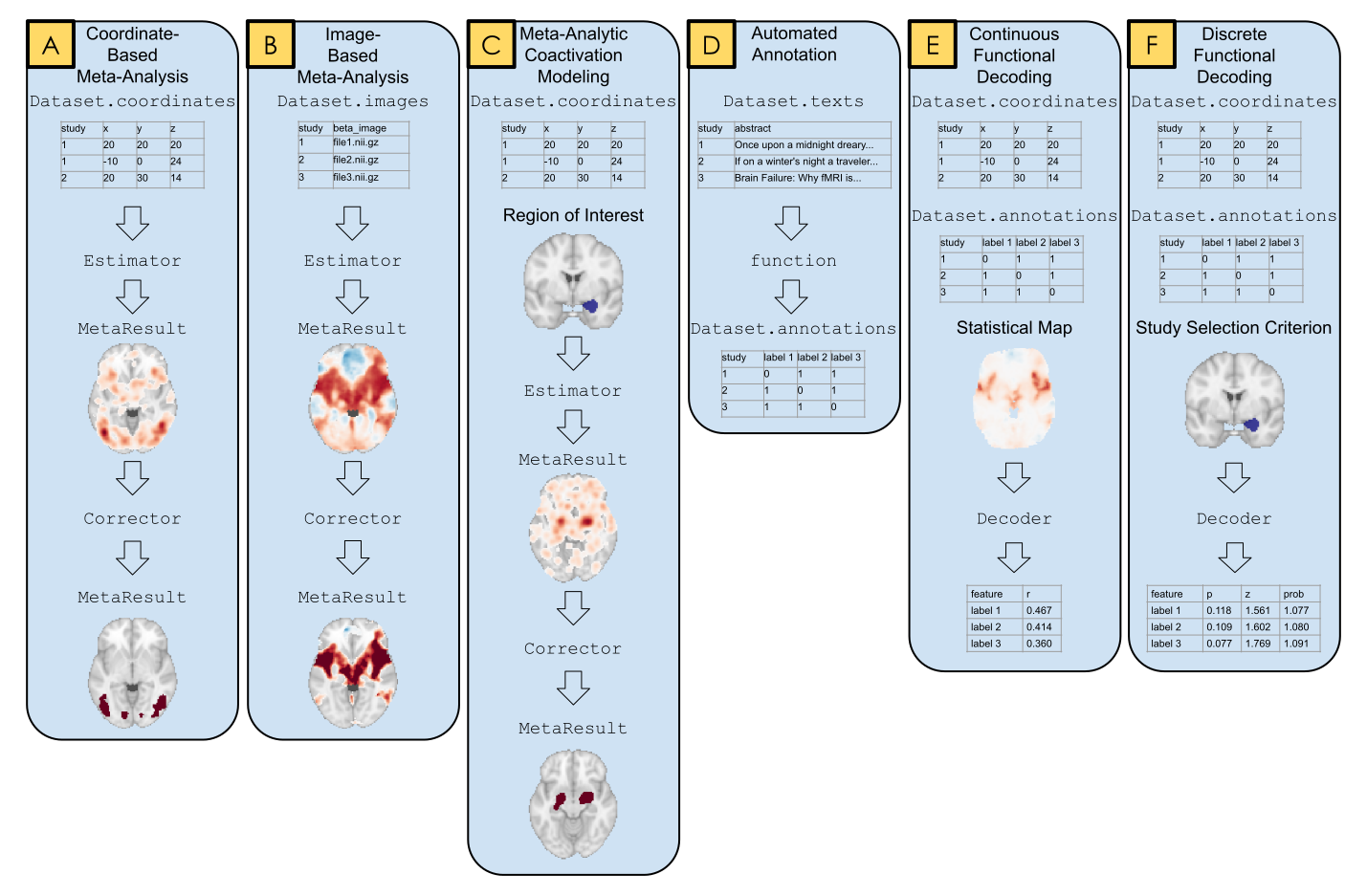
- NiMARE: Neuroimaging Meta-Analysis Research Environment
- Download the Data
- External Meta-Analytic Resources
- Coordinate-Based Meta-Analysis
- Image-Based Meta-Analysis
- Multiple Comparisons Correction
- Meta-Analytic Subtraction Analysis
- Meta-Analytic Coactivation Modeling
- Automated Annotation
- Meta-Analytic Functional Decoding
1Introduction
We introduce NiMARE (Neuroimaging Meta-Analysis Research Environment), a Python package for analyzing meta-analytic neuroimaging data. NiMARE is a new library developed as a component in a burgeoning open-source meta-analytic ecosystem for neuroimaging data, which currently includes Neurosynth, NeuroVault, NeuroQuery, and PyMARE.
While several libraries already exist for neuroimaging meta-analysis, these libraries are generally algorithm-specific, and are provided in a range of very different user interfaces, languages, and licenses. This variability may prevent meta-analysts from using the most appropriate algorithm for a given analysis. Further, having multiple meta-analysis algorithms available in one library facilitates direct comparisons of methods. With NiMARE, we consolidate meta-analytic algorithms from a range of libraries and publications, and provide a common Python syntax and well documented application program interfaces. Additionally, NiMARE is a collaboratively-developed open source package, enabling researchers to contribute new methods not included in the current version.
In this paper, we describe NiMARE’s aims, architecture and the functionality it supports—including tools for database extraction, automated annotation, meta-analysis, meta-analytic coactivation modeling, and functional decoding.
The text is accompanied by extensive code samples and results (also available online in the form of Python scripts; https://
2NiMARE Overview
NiMARE is designed to be modular and object-oriented, with an interface that mimics popular Python libraries, including scikit-learn and nilearn. This standardized interface allows users to employ a wide range of meta-analytic algorithms without having to familiarize themselves with the idiosyncrasies of algorithm-specific tools. This lets users use whatever method is most appropriate for a given research question with minimal mental overhead from switching methods. Additionally, NiMARE emphasizes citability, with references in the documentation and citable boilerplate text that can be copied directly into manuscripts, in order to ensure that the original algorithm developers are appropriately recognized.
NiMARE works with Python versions 3.6 and higher, and can easily be installed with pip.
Its source code is housed and version controlled in a GitHub repository at https://
NiMARE is under continued active development, and we anticipate that the user-facing API (application programming interface) may change over time. Our emphasis in this paper is thus primarily on reviewing the functionality implemented in the package and illustrating the general interface, and not on providing a detailed and static user guide that will be found within the package documentation.
Tools in NiMARE are organized into several modules, including nimare.meta, nimare.correct, nimare.annotate, nimare.decode, and nimare.workflows.
In addition to these primary modules, there are several secondary modules for data wrangling and internal helper functions, including nimare.io, nimare.dataset, nimare.extract, nimare.stats, nimare.utils, and nimare.base.
These modules are summarized in Section 2.1, as well as in Table 1.
2.1Application Programming Interface
One of the principal goals of NiMARE is to implement a range of methods with a set of shared interfaces, to enable users to employ the most appropriate algorithm for a given question without introducing a steep learning curve.
This approach is modeled on the widely-used scikit-learn package Pedregosa et al., 2011Buitinck et al., 2013, which implements a large number of machine learning algorithms - all with simple, consistent interfaces.
Regardless of the algorithm employed, data should be in the same format and the same class methods should be called to fit and/or generate predictions from the model.
To this end, we have adopted an object-oriented approach to NiMARE’s core API that organizes tools based on the type of inputs and outputs they operate over.
The key data structure is the nimare.dataset.Dataset class, which stores a range of neuroimaging data amenable to various forms of meta-analysis.
There are two main types of tools that operate on a Dataset class.
nimare.base.Transformer classes, as their name suggests, perform some transformation on a Dataset- i.e., they take a Dataset instance as input, and return a modified version of that Dataset instance as output (for example, with newly generated maps stored within the object).
nimare.base.Estimator classes apply a meta-analytic algorithm to a Dataset and return a set of statistical images stored in a MetaResult container class.
The key methods supported by each of these base classes, as well as the main arguments to those methods, are consistent throughout the hierarchy (e.g., all Transformer classes must implement a transform() method), minimizing the learning curve and ensuring a high degree of predictability for users.
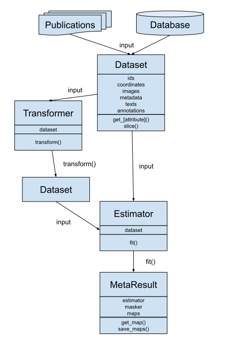
Figure 2:A schematic figure of Datasets, Estimators, Transformers, and MetaResults in NiMARE.
2.2Package Organization
At present, the package is organized into 14 distinct modules.
nimare.dataset defines the Dataset class.
nimare.meta includes Estimators for coordinate- and image-based meta-analysis methods.
nimare.results defines the MetaResult class, which stores statistical maps produced by meta-analyses.
nimare.correct implements Corrector classes for family-wise error (FWE) and false discovery rate (FDR) multiple comparisons correction.
nimare.annotate implements a range of automated annotation methods, including latent Dirichlet allocation (LDA) and generalized correspondence latent Dirichlet allocation (GCLDA).
nimare.decode implements a number of meta-analytic functional decoding and encoding algorithms.
nimare.io provides functions for converting alternative meta-analytic dataset structure, such as Sleuth text files or Neurosynth datasets, to NiMARE format.
nimare.transforms implements a range of spatial and data type transformations, including a function to generate new images in the Dataset from existing image types.
nimare.extract provides methods for fetching datasets and models across the internet.
nimare.generate includes functions for generating data for internal testing and validation.
nimare.base defines a number of base classes used throughout the rest of the package.
Finally, nimare.stats and nimare.utils are modules for statistical and generic utility functions, respectively.
These modules are summarized in Table 1.
Table 1:Summaries of modules in NiMARE.
| Module | Description |
|---|---|
dataset | This module stores the Dataset class, which contains NiMARE datasets. |
meta | This module contains Estimators for image- and coordinate-based meta-analysis algorithms, as well as KernelTransformers, which are used in conjunction with coordinate-based methods. |
results | This module stores the MetaResult class, which in turn is used to manage statistical maps produced by meta-analytic algorithms. |
correct | This module contains classes for multiple comparisons correction, including FWECorrector (family-wise error rate correction) and FDRCorrector (false discovery rate correction). |
annotate | This module includes a range of tools for automated annotation of studies. Methods in this module include: topic models, such as latent Dirichlet allocation and generalized correspondence latent Dirichlet allocation; ontology-based annotation, such as Cognitive Atlas term extract from text; and general text-based feature extraction, such as count or tf-idf extraction from text. |
decode | This module includes a number of methods for functional characterization analysis, also known as functional decoding. Methods in this module are divided into three groups: discrete, for decoding regions of interest or subsets of the Dataset; continuous, for decoding unthresholded statistical maps; and encoding, for simulating statistical maps from labels. |
io | This module contains functions for converting common file types, such as Neurosynth- or Sleuth-format files, into NiMARE-compatible formats, such as Dataset objects. |
transforms | This module contains classes and functions for converting between common data types. Two important classes in this module are the ImageTransformer, which uses available images and metadata to produce new images in a Dataset, and the ImagesToCoordinates, which extracts peak coordinates from images in the Dataset, so that image-based studies can be used for coordinate-based meta-analyses. |
extract | This module contains functions for downloading external resources, such as the Neurosynth dataset and the Cognitive Atlas ontology. |
stats | This module contains miscellaneous statistical methods used throughout the rest of the library. |
generate | This module contains functions for generating useful data for internal testing and validation. |
utils | This module contains miscellaneous utility functions used throughout the rest of the library. |
workflows | This module contains a number of common workflows that can be run from the command line, such as an ALE meta-analysis or a contrast-permutation image-based meta-analysis. All of the workflow functions additionally generate boilerplate text that can be included in manuscript methods sections. |
base | This module defines a number of base classes used throughout the rest of the library. |
2.3Dependencies
NiMARE depends on the standard SciPy stack, as well as a small number of widely-used packages.
Dependencies from the SciPy stack include scipy Virtanen et al., 2020, numpy Walt et al., 2011Harris et al., 2020, pandas McKinney, 2010, and scikit-learn Pedregosa et al., 2011Buitinck et al., 2013.
Additional requirements include fuzzywuzzy, nibabel Brett et al., 2020, nilearn Abraham et al., 2014, statsmodels Seabold & Perktold, 2010, and tqdm Costa-Luis et al., 2020.
3Download the Data
We will also create a directory in which to save files that are generated within the book.
4External Meta-Analytic Resources
Large-scale meta-analytic databases have made systematic meta-analyses of the neuroimaging literature possible. These databases combine results from neuroimaging studies, whether represented as coordinates of peak activations or unthresholded statistical images, with important study metadata, such as information about the samples acquired, stimuli used, analyses performed, and mental constructs putatively manipulated. The two most popular coordinate-based meta-analytic databases are BrainMap and Neurosynth, while the most popular image-based database is NeuroVault.
The studies archived in these databases may be either manually or automatically annotated—often with reference to a formal ontology or controlled vocabulary. Ontologies for cognitive neuroscience define what mental states or processes are postulated to be manipulated or measured in experiments, and may also include details of said experiments (e.g.,the cognitive tasks employed), relationships between concepts (e.g., verbal working memory is a kind of working memory), and various other metadata that can be standardized and represented in a machine-readable form Poldrack & Yarkoni, 2016Poldrack, 2010Turner & Laird, 2012. Some of these ontologies are very well-defined, such as expert-generated taxonomies designed specifically to describe only certain aspects of experiments and the relationships between elements within the taxonomy, while others are more loosely defined, in some cases simply building a vocabulary based on which terms are commonly used in cognitive neuroscience articles.
4.1BrainMap
BrainMap Fox et al., 2005Fox & Lancaster, 2002Laird et al., 2005 relies on expert annotators to label individual comparisons within studies according to its internally developed ontology, the BrainMap Taxonomy Fox et al., 2005. While this approach is likely to be less noisy than an automated annotation method using article text or imaging results to predict content, it is also subject to a number of limitations. First, there are simply not enough annotators to keep up with the ever-expanding literature. Second, any development of the underlying ontology has the potential to leave the database outdated. For example, if a new label is added to the BrainMap Taxonomy, then each study in the full BrainMap database needs to be evaluated for that label before that label can be properly integrated into the database. Finally, a manually annotated database like BrainMap will be biased by which subdomains within the literature are annotated. While outside contributors can add and annotate studies to the database, the main source of annotations has been researchers associated with the BrainMap project.
While BrainMap is a semi-closed resource (i.e., a collaboration agreement is required to access the full database), registered users may search the database using the Sleuth search tool, in order to collect samples for meta-analyses. Sleuth can export these study collections as text files with coordinates. NiMARE provides a function to import data from Sleuth text files into the NiMARE Dataset format.
The function nimare.io.convert_sleuth_to_dataset can be used to convert text files exported from Sleuth into NiMARE Datasets.
Here, we convert two files from a previous publication by NiMARE contributors Yanes et al., 2018 into two separate Datasets.
4.2Neurosynth
Neurosynth Yarkoni et al., 2011 uses a combination of web scraping and text mining to automatically harvest neuroimaging studies from the literature and to annotate them based on term frequency within article abstracts. As a consequence of its relatively crude automated approach, Neurosynth has its own set of limitations. First, Neurosynth is unable to delineate individual comparisons within studies, and consequently uses the entire paper as its unit of measurement, unlike BrainMap. This risks conflating directly contrasted comparisons (e.g., A>B and B>A), as well as comparisons which have no relation to one another. Second, coordinate extraction and annotation are noisy. Third, annotations automatically performed by Neurosynth are also subject to error, although the reasons behind this are more nuanced and will be discussed later in this paper. Given Neurosynth’s limitations, we recommend that it be used for casual, exploratory meta-analyses rather than for publication-quality analyses. Nevertheless, while individual meta-analyses should not be published from Neurosynth, many derivative analyses have been performed and published (e.g., Chang et al., 2013Vega et al., 2016Vega et al., 2018Poldrack et al., 2012). As evidence of its utility, Neurosynth has been used to define a priori regions of interest (e.g., Josipovic, 2014Zeidman et al., 2012Wager et al., 2013) or perform meta-analytic functional decoding (e.g., Chen et al., 2018Pantelis et al., 2015Tambini et al., 2017) in many first-order (rather than meta-analytic) fMRI studies.
Here, we show code that would download the Neurosynth database from where it is stored (https://Dataset using nimare.extract.fetch_neurosynth, for the first step, and nimare.io.convert_neurosynth_to_dataset, for the second.
# Convert the files to a Dataset.

# This may take a while (~10 minutes)

neurosynth_dset = io.convert_neurosynth_to_dataset(
    coordinates_file=neurosynth_db["coordinates"],
    metadata_file=neurosynth_db["metadata"],
    annotations_files=neurosynth_db["features"],
)
print(neurosynth_dset)

# Save the Dataset for later use.

neurosynth_dset.save(os.path.join(out_dir, "neurosynth_dataset.pkl.gz"))
Here, we load a pre-generated version of the Neurosynth Dataset.
In addition to a large corpus of coordinates, Neurosynth provides term frequencies derived from article abstracts that can be used as annotations.
One additional benefit to Neurosynth is that it has made available the coordinates for a large number of studies for which the study abstracts are also readily available. This has made the Neurosynth database a common resource upon which to build other automated ontologies. Data-driven ontologies which have been developed using the Neurosynth database include the generalized correspondence latent Dirichlet allocation (GCLDA) Rubin et al., 2017 topic model and Deep Boltzmann machines Monti et al., 2016.
4.3NeuroQuery
A related resource is NeuroQuery Dockès et al., 2020. NeuroQuery is an online service for large-scale predictive meta-analysis. Unlike Neurosynth, which performs statistical inference and produces statistical maps, NeuroQuery is a supervised learning model and produces a prediction of the brain areas most likely to contain activations. These maps predict locations where studies investigating a given area (determined by the text prompt) are likely to produce activations, but they cannot be used in the same manner as statistical maps from a standard coordinate-based meta-analysis. In addition to this predictive meta-analytic tool, NeuroQuery also provides a new database of coordinates, text annotations, and metadata via an automated extraction approach that improves on Neurosynth’s original methods.
While NiMARE does not currently include an interface to NeuroQuery’s predictive meta-analytic method, there are functions for downloading the NeuroQuery database and converting it to NiMARE format, much like Neurosynth.
The functions for downloading the NeuroQuery database and converting it to a Dataset are nimare.extract.fetch_neuroquery and nimare.io.convert_neurosynth_to_dataset, respectively.
We are able to use the same function for converting the database to a Dataset for NeuroQuery as Neurosynth because both databases store their data in the same structure.
# Convert the files to a Dataset.

# This may take a while (~10 minutes)

neuroquery_dset = io.convert_neurosynth_to_dataset(
    coordinates_file=neuroquery_db["coordinates"],
    metadata_file=neuroquery_db["metadata"],
    annotations_files=neuroquery_db["features"],
)
print(neuroquery_dset)

# Save the Dataset for later use.

neuroquery_dset.save(os.path.join(out_dir, "neuroquery_dataset.pkl.gz"))
Here, we load a pre-generated version of the NeuroQuery Dataset.
4.4NeuroVault
NeuroVault Gorgolewski et al., 2015 is a public repository of user-uploaded, whole-brain, unthresholded brain maps.
Users may associate their image collections with publications, and can annotate individual maps with labels from the Cognitive Atlas, which is the ontology of choice for NeuroVault.
NiMARE includes a function, nimare.io.convert_neurovault_to_dataset, with which users can search for images in NeuroVault, download those images, and convert them into a Dataset object.
5Coordinate-Based Meta-Analysis
Coordinate-based meta-analysis (CBMA) is currently the most popular method for neuroimaging meta-analysis, given that the majority of fMRI papers currently report their findings as peaks of statistically significant clusters in standard space and do not release unthresholded statistical maps. These peaks indicate where significant results were found in the brain, and thus do not reflect an effect size estimate for each hypothesis test (i.e., each voxel) as one would expect for a typical meta-analysis. As such, standard methods for effect size-based meta-analysis cannot be applied. Over the past two decades, a number of algorithms have been developed to determine whether peaks converge across experiments in order to identify locations of consistent or specific activation associated with a given hypothesis Samartsidis et al., 2017Müller et al., 2018.
Kernel-based methods evaluate convergence of coordinates across studies by first convolving foci with a spatial kernel to produce study-specific modeled activation maps, then combining those modeled activation maps into a sample-wise map, which is compared to a null distribution to evaluate voxel-wise statistical significance. Additionally, for each of the following approaches, except for SCALE, voxel- or cluster-level multiple comparisons correction may be performed using Monte Carlo simulations or false discovery rate (FDR) Laird et al., 2005 correction. Basic multiple-comparisons correction methods (e.g., Bonferroni correction) are also supported.
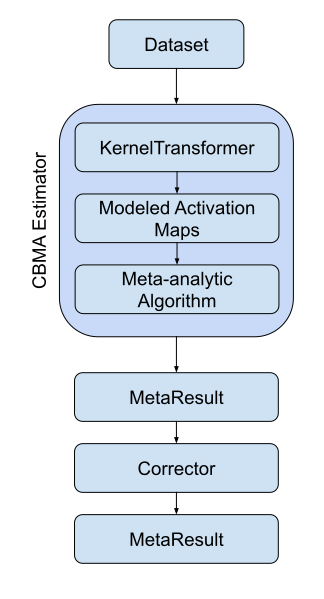
Figure 3:A flowchart of the typical workflow for coordinate-based meta-analyses in NiMARE.
5.1CBMA kernels
CBMA kernels are available as nimare.meta.kernel.KernelTransformers in the nimare.meta.kernel module.
There are three standard kernels that are currently available: nimare.meta.kernel.MKDAKernel, nimare.meta.kernel.KDAKernel, and nimare.meta.kernel.ALEKernel.
Each class may be configured with certain parameters when a new object is initialized.
For example, MKDAKernel accepts an r parameter, which determines the radius of the spheres that will be created around each peak coordinate.
ALEKernel automatically uses the sample size associated with each experiment in the Dataset to determine the appropriate full-width-at-half-maximum of its Gaussian distribution, as described in Eickhoff et al. (2012); however, users may provide a constant sample_size or fwhm parameter when sample size information is not available within the Dataset metadata.
Here we show how these three kernels can be applied to the same Dataset.
/srv/conda/envs/notebook/lib/python3.7/site-packages/nilearn/plotting/img_plotting.py:348: FutureWarning: Default resolution of the MNI template will change from 2mm to 1mm in version 0.10.0
  anat_img = load_mni152_template()
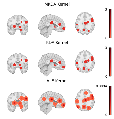
Figure 4:Modeled activation maps produced by NiMARE’s KernelTransformer classes.
5.2Multilevel kernel density analysis
Multilevel kernel density analysis (MKDA) Wager et al., 2007 is a kernel-based method that convolves each peak from each study with a binary sphere of a set radius. These peak-specific binary maps are then combined into study-specific maps by taking the maximum value for each voxel. Study-specific maps are then averaged across the meta-analytic sample. This averaging is generally weighted by studies’ sample sizes, although other covariates may be included, such as weights based on the type of inference (random or fixed effects) employed in the study’s analysis. An arbitrary threshold is generally employed to zero-out voxels with very low values, and then a Monte Carlo procedure is used to assess statistical significance, either at the voxel or cluster level.
In NiMARE, the MKDA meta-analyses can be performed with the nimare.meta.cbma.mkda.MKDADensity class.
This class, like most other CBMA classes in NiMARE, accepts a null_method parameter, which determines how voxel-wise (uncorrected) statistical significance is calculated.
Here we perform an MKDADensity meta-analysis on one of the Sleuth-based Datasets. We will use the “approximate” null method for speed.
5.2.1The MetaResult class
Fitting an Estimator to a Dataset produces a nimare.results.MetaResult object.
The MetaResult class is a light container holding the different statistical maps produced by the Estimator.
This result is also retained as an attribute in the Estimator.
The maps attribute is a dictionary containing statistical map names and associated numpy arrays.
These arrays can be transformed into image-like objects using the masker attribute.
We can also use the get_map method to get that image object.
We can save the statistical maps to an output directory as gzipped nifti files, with a prefix. Here, we will save all of the statistical maps with the MKDADensity prefix.
We will also save the Estimator itself, which we will reuse when we get to multiple comparisons correction.
Since this is a kernel-based algorithm, the kernel transformer is an optional input to the meta-analytic estimator, and can be controlled in a more fine-grained manner.
5.3Kernel density analysis
Kernel density analysis (KDA) Wager et al., 2003Wager et al., 2004 is a precursor algorithm that has been replaced in the field by MKDA. For the sake of completeness, NiMARE also includes a KDA estimator that implements the older KDA algorithm for comparison purposes. The interface is virtually identical, but since there are few if any legitimate uses of KDA (which models studies as fixed rather than random effects), we do not discuss the algorithm further here.
5.4Activation likelihood estimation
Activation likelihood estimation (ALE) Eickhoff et al., 2012Turkeltaub et al., 2012Turkeltaub et al., 2002 assesses convergence of peaks across studies by first generating a modeled activation map for each study, in which each of the experiment’s peaks is convolved with a 3D Gaussian distribution determined by the experiment’s sample size, and then by combining these modeled activation maps across studies into an ALE map, which is compared to an empirical null distribution to assess voxel-wise statistical significance.
5.5Specific coactivation likelihood estimation
Specific coactivation likelihood estimation (SCALE) Langner et al., 2014 is an extension of the ALE algorithm developed for meta-analytic coactivation modeling (MACM) analyses. Rather than comparing convergence of foci within the sample to a null distribution derived under the assumption of spatial randomness within the brain, SCALE assesses whether the convergence at each voxel is greater than in the general literature. Each voxel in the brain is assigned a null distribution determined based on the base rate of activation for that voxel across an existing coordinate-based meta-analytic database. This approach allows for the generation of a statistical map for the sample, but no methods for multiple comparisons correction have yet been developed. While this method was developed to support analysis of joint activation or “coactivation” patterns, it is generic and can be applied to any CBMA; see
5.6MKDA Chi-Squared Analysis
An alternative to the density-based approaches (i.e., MKDA, KDA, ALE, and SCALE) is the MKDA Chi-squared extension Wager et al., 2007. Though still a kernel-based method in which foci are convolved with a binary sphere and combined within studies, this approach uses voxel-wise chi-squared tests to assess both consistency (i.e., higher convergence of foci within the meta-analytic sample than expected by chance) and specificity (i.e., higher convergence of foci within the meta-analytic sample than detected in an unrelated dataset) of activation. Such an analysis also requires access to a reference meta-analytic sample or database of studies. For example, to perform a chi-squared analysis of working memory studies, the researcher will also need a comprehensive set of studies which did not manipulate working memory—ideally one that is matched with the working memory study set on all relevant attributes except the involvement of working memory.
5.7Comparing algorithms
Here we load the z-statistic map from each of the CBMA Estimators we’ve used throughout this chapter and plot them all side by side.
Output
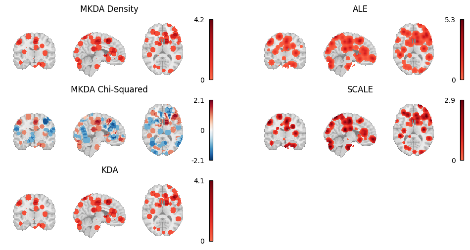
Figure 5:Thresholded results from MKDA Density, KDA, ALE, and SCALE meta-analyses.
A number of other coordinate-based meta-analysis algorithms exist which are not yet implemented in NiMARE. We describe these algorithms briefly in .
6Image-Based Meta-Analysis
Image-based meta-analysis (IBMA) methods perform a meta-analysis directly on brain images (either whole-brain or partial) rather than on extracted peaks. On paper, IBMA is superior to CBMA in virtually all respects, as the availability of analysis-level parameter and variance estimates at all analyzed voxels allows researchers to use the full complement of standard meta-analysis techniques, instead of having to resort to kernel-based or other methods that require additional spatial assumptions. In principle, given a set of maps that contains no missing values (i.e., where there are k valid pairs of parameter and variance estimates at each voxel), one can simply conduct a voxel-wise version of any standard meta-analysis or meta-regression method commonly used in other biomedical or social science fields.
In practice, the utility of IBMA methods has historically been quite limited, as unthresholded statistical maps have been unavailable for the vast majority of neuroimaging studies. However, the introduction and rapid adoption of NeuroVault Gorgolewski et al., 2015, a database for unthresholded statistical images, has made image-based meta-analysis increasingly viable. Although coverage of the literature remains limited, and IBMAs of maps drawn from the NeuroVault database are likely to omit at least some (and in some cases most) relevant studies due to limited metadata, we believe the time is ripe for researchers to start including both CBMAs and IBMAs in published meta-analyses, with the aspirational goal of eventually transitioning exclusively to the latter. To this end, NiMARE supports a range of different IBMA methods, including a number of estimators of the gold standard mixed-effects meta-regression model, as well as several alternative estimators suitable for use when some of the traditional inputs are unavailable.
In the optimal situation, meta-analysts have access to both contrast (i.e., parameter estimate) maps and their associated standard error maps for a number of studies. With these data, researchers can fit the traditional random-effects meta-regression model using one of several methods that vary in the way they estimate the between-study variance (). Currently supported estimators include the DerSimonian-Laird method DerSimonian & Laird, 1986, the Hedges method Hedges et al., 1985, and maximum-likelihood (ML) and restricted maximum-likelihood (REML) approaches. NiMARE can also perform fixed-effects meta-regression via weighted least-squares, though there are few IBMA scenarios where a fixed-effects analysis would be indicated. It is worth noting that the non-likelihood-based estimators (i.e., DerSimonian-Laird and Hedges) have a closed-form solution, and are implemented in an extremely efficient way in NiMARE (i.e., computation is performed on all voxels in parallel). However, these estimators also produce more biased estimates under typical conditions (e.g., when sample sizes are very small), implying a tradeoff from the user’s perspective.
Alternatively, when users only have access to contrast maps and associated sample sizes, they can use the supported Sample Size-Based Likelihood estimator, which assumes that within-study variance is constant across studies, and uses maximum-likelihood or restricted maximum-likelihood to estimate between-study variance, as described in Sangnawakij et al. (2019). When users have access only to contrast maps, they can use the Permuted OLS estimator, which uses ordinary least squares and employs a max-type permutation scheme for family-wise error correction Freedman & Lane, 1983Anderson & Robinson, 2001 that has been validated on neuroimaging data Winkler et al., 2014 and relies on the nilearn library.
Finally, when users only have access to z-score maps, they can use either the Fisher’s Fisher, 1925 or the Stouffer’s Riley et al., 1949 estimators. When sample size information is available, users may incorporate that information into the Stouffer’s method, via the method described in Zaykin (2011).
Given the paucity of image-based meta-analytic datasets, we have included the tools to build a Dataset from a NeuroVault collection of 21 pain studies, originally described in Maumet & Nichols (2016).
6.1Transforming images
Researchers may share their statistical maps in many forms, some of which are direct transformations of one another.
For example, researchers may share test statistic maps with z-statistics or t-statistics, and, as long as we know the degrees of freedom associated with the t-test, we can convert between the two easily. To that end, NiMARE includes a class, nimare.transforms.ImageTransformer, which will calculate target image types from available ones, as long as the available images are compatible with said transformation.
Here, we use ImageTransformer to calculate z-statistic and variance maps for all studies with compatible images.
This allows us to apply more image-based meta-analysis algorithms to the Dataset.
Now that we have filled in as many gaps in the Dataset as possible, we can start running meta-analyses.
We will start with a DerSimonian-Laird meta-analysis (nimare.meta.ibma.DerSimonianLaird).
Now we will apply other available IBMA Estimators to the same Dataset, and save their results to files for comparison.
6.2Comparing algorithms
Here we load the z-statistic map from each of the IBMA Estimators we’ve used throughout this chapter and plot them all side by side.
Output
/srv/conda/envs/notebook/lib/python3.7/site-packages/nilearn/plotting/img_plotting.py:348: FutureWarning: Default resolution of the MNI template will change from 2mm to 1mm in version 0.10.0
  anat_img = load_mni152_template()
/srv/conda/envs/notebook/lib/python3.7/site-packages/nilearn/_utils/niimg.py:62: UserWarning: Non-finite values detected. These values will be replaced with zeros.
  "Non-finite values detected. "
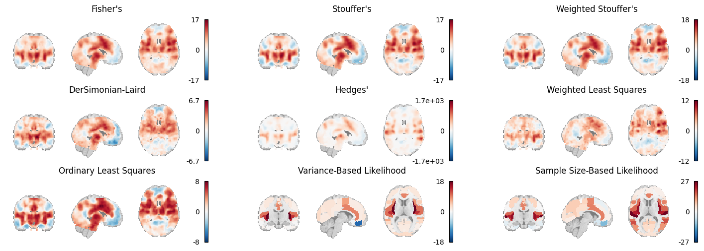
Figure 6:An array of plots of the statistical maps produced by the image-based meta-analysis methods. The likelihood-based meta-analyses are run on atlases instead of voxelwise.
7Multiple Comparisons Correction
In NiMARE, multiple comparisons correction is separated from each CBMA and IBMA Estimator, so that any number of relevant correction methods can be applied after the Estimator has been fit to the Dataset.
Some correction options, such as the montecarlo option for FWE correction, are designed to work specifically with a given Estimator (and are indeed implemented within the Estimator class, and only called by the Corrector).
Correctors are divided into two subclasses: FWECorrectors, which correct based on family-wise error rate, and FDRCorrectors, which correct based on false discovery rate.
All Correctors are initialized with a number of parameters, including the correction method that will be used.
After that, you can use the transform method on a MetaResult object produced by a CBMA or IBMA Estimator to apply the correction method.
This will return an updated MetaResult object, with both the statistical maps from the original MetaResult, as well as new, corrected maps.
Here we will apply both FWE and FDR correction to results from a MKDADensity meta-analysis, performed back in Section 5.2.
Statistical maps saved by NiMARE MetaResults automatically follow a naming convention based loosely on the Brain Imaging Data Standard (BIDS).
Let’s take a look at the files created by the FWECorrector.
If you ignore the prefix, which was specified in the call to MetaResult.save_maps, the maps all have a common naming convention.
The maps from the original meta-analysis (before multiple comparisons correction) are simply named according to the values contained in the map (e.g., z, stat, p).
Maps generated by the correction method, however, use a series of key-value pairs to indicate how they were generated.
The corr key indicates whether FWE or FDR correction was applied.
The method key reflects the correction method employed, which was defined by the method parameter used to create the Corrector.
The level key simply indicates if the map was corrected at the voxel or cluster level.
Finally, the desc key reflects any necessary description that goes beyond what is already covered by the other entities.
/srv/conda/envs/notebook/lib/python3.7/site-packages/nilearn/plotting/img_plotting.py:348: FutureWarning: Default resolution of the MNI template will change from 2mm to 1mm in version 0.10.0
  anat_img = load_mni152_template()
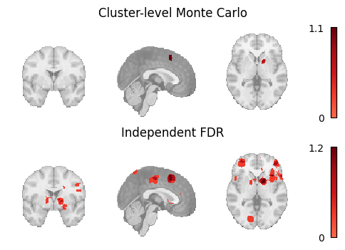
Figure 7:An array of plots of the corrected statistical maps produced by the different multiple comparisons correction methods.
8Derivative Analyses
Meta-analytic databases and algorithms may be employed for derivative analyses, including subtraction analysis, meta-analytic coactivation modeling (MACM), meta-analytic clustering, coactivation-based parcellation (CBP), meta-analytic independent component analysis (meta-ICA), semantic model development, and meta-analytic functional decoding. In this part, we describe the derivative analyses implemented in NiMARE and include examples of use cases.
9Meta-Analytic Subtraction Analysis
Subtraction analysis refers to the voxel-wise comparison of two meta-analytic samples. In image-based meta-analysis, comparisons between groups of maps can generally be accomplished within the standard meta-regression framework (i.e., by adding a covariate that codes for group membership). However, coordinate-based subtraction analysis requires special extensions for CBMA algorithms.
Subtraction analysis to compare the results of two ALE meta-analyses was originally implemented by Laird et al. (2005) and later extended by Eickhoff et al. (2012). In this approach, two groups of experiments (A and B) are compared using a group assignment randomization procedure in which voxel-wise null distributions are generated by randomly reassigning experiments between the two groups and calculating ALE-difference scores for each permutation. Real ALE-difference scores (i.e., the ALE values for one group minus the ALE values for the other) are compared against these null distributions to determine voxel-wise significance. In the original implementation of the algorithm, this procedure is performed separately for a group A > B contrast and a group B > A contrast, where each contrast is limited to voxels that were significant in the first group’s original meta-analysis.
/srv/conda/envs/notebook/lib/python3.7/site-packages/nilearn/plotting/img_plotting.py:348: FutureWarning: Default resolution of the MNI template will change from 2mm to 1mm in version 0.10.0
  anat_img = load_mni152_template()
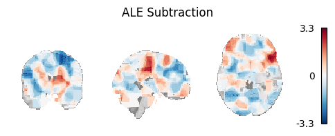
Figure 8:Unthresholded z-statistic map for the subtraction analysis of the two example Sleuth-based Datasets.
Alternatively, MKDA Chi-squared analysis is inherently a subtraction analysis method, in that it compares foci from two groups of studies. Generally, one of these groups is a sample of interest, while the other is a meta-analytic database (minus the studies in the sample). With this setup, meta-analysts can infer whether there is greater convergence of foci in a voxel as compared to the baseline across the field (as estimated with the meta-analytic database), much like SCALE. However, if the database is replaced with a second sample of interest, the analysis ends up comparing convergence between the two groups.
10Meta-Analytic Coactivation Modeling
Meta-analytic coactivation modeling (MACM) Laird et al., 2009Robinson et al., 2010Eickhoff et al., 2010, also known as meta-analytic connectivity modeling, uses meta-analytic data to measure co-occurrence of activations between brain regions providing evidence of functional connectivity of brain regions across tasks. In coordinate-based MACM, whole-brain studies within the database are selected based on whether or not they report at least one peak in a region of interest specified for the analysis. These studies are then subjected to a meta-analysis, often comparing the selected studies to those remaining in the database. In this way, the significance of each voxel in the analysis corresponds to whether there is greater convergence of foci at the voxel among studies which also report foci in the region of interest than those which do not.
MACM results have historically been accorded a similar interpretation to task-related functional connectivity (e.g., Hok et al., 2015Kellermann et al., 2013), although this approach is quite removed from functional connectivity analyses of task fMRI data (e.g., beta-series correlations, psychophysiological interactions, or even seed-to-voxel functional connectivity analyses on task data). Nevertheless, MACM analyses do show high correspondence with resting-state functional connectivity Reid et al., 2017. MACM has been used to characterize the task-based functional coactivation of the cerebellum Riedel et al., 2015, lateral prefrontal cortex Reid et al., 2016, fusiform gyrus Caspers et al., 2014, and several other brain regions.
Within NiMARE, MACMs can be performed by selecting studies in a Dataset based on the presence of activation within a target mask or coordinate-centered sphere. While some algorithms, such as SCALE, may have been designed with MACMs in mind, in practice MACMs may be performed with any valid Estimator.
In this section, we will perform two MACMs- one with a target mask and one with a coordinate-centered sphere.
For the former, we use nimare.dataset.Dataset.get_studies_by_mask.
For the latter, we use nimare.dataset.Dataset.get_studies_by_coordinate.
/srv/conda/envs/notebook/lib/python3.7/site-packages/nilearn/plotting/img_plotting.py:348: FutureWarning: Default resolution of the MNI template will change from 2mm to 1mm in version 0.10.0
  anat_img = load_mni152_template()
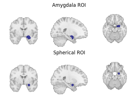
Figure 9:Region of interest masks for (1) a target mask-based MACM and (2) a coordinate-based MACM.
Once the Dataset has been reduced to studies with coordinates within the mask or sphere requested, any of the supported CBMA Estimators can be run.
Figure 10:Unthresholded z-statistic maps for (1) the target mask-based MACM and (2) the coordinate-based MACM.
11Automated Annotation
As mentioned in the discussion of BrainMap (Section 4.1), manually annotating studies in a meta-analytic database can be a time-consuming and labor-intensive process. To facilitate more efficient (albeit lower-quality) annotation, NiMARE supports a number of automated annotation approaches. These include Section 11.1, Section 11.2, Section 11.3, and Section 11.4.
NiMARE users may download abstracts from PubMed as long as study identifiers in the Dataset correspond to PubMed IDs (as in Neurosynth and NeuroQuery).
Abstracts are much more easily accessible than full article text, so most annotation methods in NiMARE rely on them.
Below, we use the function nimare.extract.download_abstracts to download abstracts for the Neurosynth Dataset.
This will attempt to extract metadata about each study in the Dataset from PubMed, and then add the abstract available on Pubmed to the Dataset’s texts attribute, under a new column names “abstract”.
# First, load a Dataset without abstracts

neurosynth_dset_first_500 = dataset.Dataset.load(
    os.path.join(data_path, "neurosynth_dataset_first500.pkl.gz")
)

# Now, download the abstracts using your email address

neurosynth_dset_first_500 = extract.download_abstracts(
    neurosynth_dset_first_500,
    email="example@email.com",
)

# Finally, save the Dataset with abstracts to a pkl.gz file

neurosynth_dset_first_500.save(
    os.path.join(data_path, "neurosynth_dataset_first500_with_abstracts.pkl.gz"),
)11.1N-gram term extraction
N-gram term extraction refers to the vectorization of text into contiguous sets of words that can be counted as individual tokens. The upper limit on the number of words in these tokens is set by the user.
NiMARE has the function nimare.annotate.text.generate_counts to extract n-grams from text.
This method produces either term counts or term frequency- inverse document frequency (tf-idf) values for each of the studies in a Dataset.
This term count DataFrame will be used later, to train a GCLDA model.
11.2Cognitive Atlas term extraction and hierarchical expansion
Cognitive Atlas term extraction leverages the structured nature of the Cognitive Atlas in order to extract counts for individual terms and their synonyms in the ontology, as well as to apply hierarchical expansion to these counts based on the relationships specified between terms. This method produces both basic term counts and expanded term counts based on the weights applied to different relationship types present in the ontology.
First, we must use nimare.extract.download_cognitive_atlas to download the current version of the Cognitive Atlas ontology.
This includes both information about individual terms in the ontology and asserted relationships between those terms.
NiMARE will automatically attempt to extrapolate likely alternate forms of each term in the ontology, in order to make extraction easier. For an example, see Figure 11.
Figure 11:An example of alternate forms characterized by the Cognitive Atlas and extrapolated by NiMARE. Certain alternate forms (i.e., synonyms) are specified within the Cognitive Atlas, while others are inferred automatically by NiMARE according to certain rules (e.g., removing parentheses).
Output
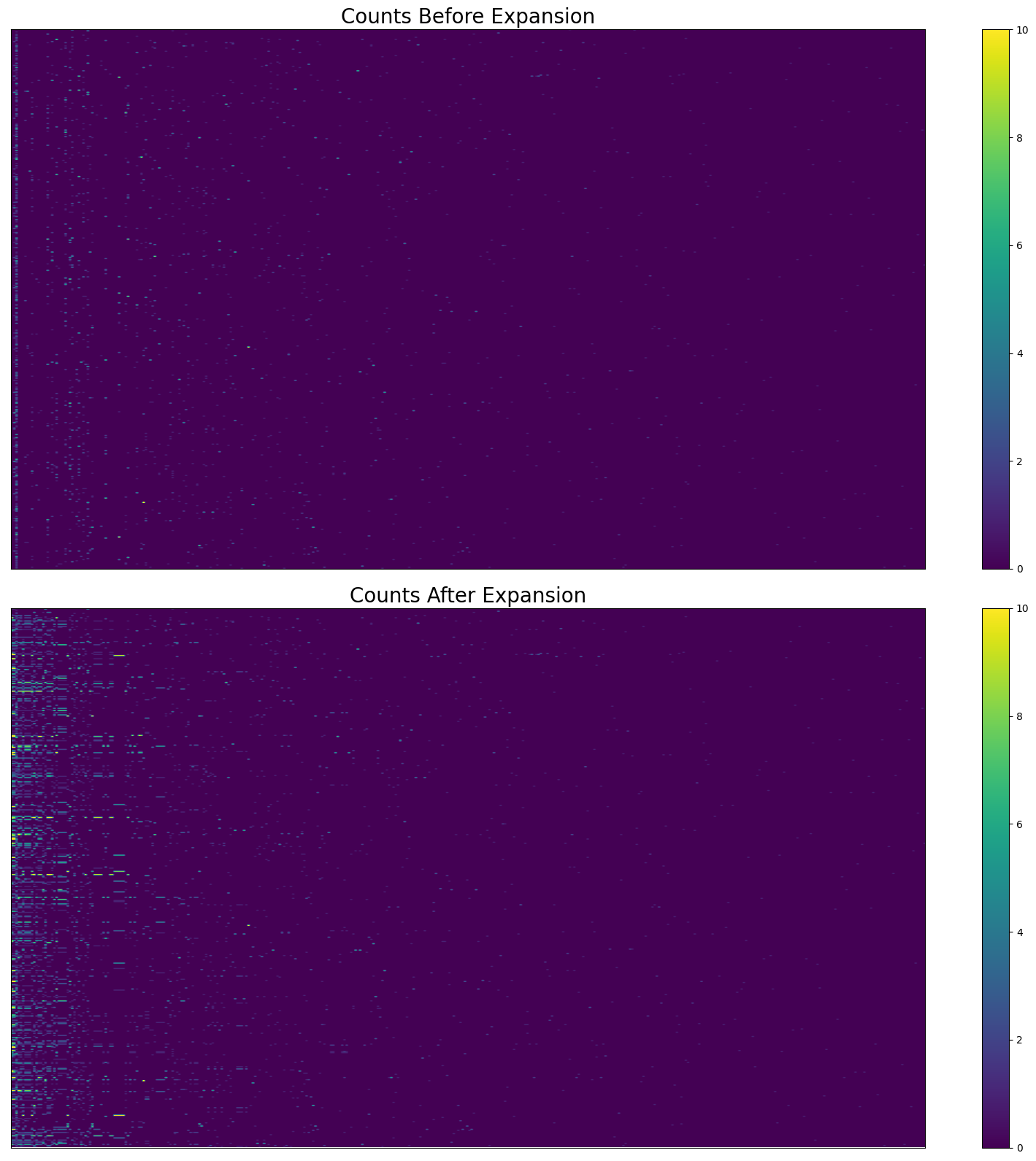
Figure 12:The effect of hierarchical expansion on Cognitive Atlas term counts from abstracts in Neurosynth’s first 500 papers. There are too many terms and studies to show individual labels.
11.3Latent Dirichlet allocation
Latent Dirichlet allocation (LDA) Blei et al., 2003 was originally combined with meta-analytic neuroimaging data in Poldrack et al. (2012). LDA is a generative topic model which, for a text corpus, builds probability distributions across documents and words. In LDA, each document is considered a mixture of topics. This works under the assumption that each document was constructed by first randomly selecting a topic based on the document’s probability distribution across topics, and then randomly selecting a word from that topic based on the topic’s probability distribution across words. While this is not a useful generative model for producing documents, LDA is able to discern cohesive topics of related words. Poldrack et al. (2012) were able to apply LDA to full texts from neuroimaging articles in order to develop cognitive neuroscience-related topics and to run topic-wise meta-analyses. This method produces two sets of probability distributions: (1) the probability of a word given topic and (2) the probability of a topic given article.
NiMARE’s nimare.annotate.lda.LDAModel is a light wrapper around scikit-learn’s LDA implementation.
Here, we train an LDA model (nimare.annotate.lda.LDAModel) on the first 500 studies of the Neurosynth Dataset, with 50 topics in the model.
The most important products of training the LDAModel object is its distributions_ attribute.
LDAModel.distributions_ is a dictionary containing arrays and DataFrames created from training the model.
We are particularly interested in the p_topic_g_word_df distribution, which is a pandas DataFrame in which each row corresponds to a topic and each column corresponds to a term (n-gram) extracted from the Dataset’s texts.
The cells contain weights indicating the probability distribution across terms for each topic.
Additionally, the LDAModel updates the Dataset’s nimare.dataset.Dataset.annotations attribute, by adding columns corresponding to each of the topics in the model.
Each study in the Dataset thus receives a weight for each topic, which can be used to select studies for topic-based meta-analyses or functional decoding.
Let’s take a look at the results of the model training. First, we will reorganize the DataFrame a bit to show the top ten terms for each of the first ten topics.
Output
Figure 13:The top ten terms for each of the first ten topics in the trained LDA model.
11.4Generalized correspondence latent Dirichlet allocation
Generalized correspondence latent Dirichlet allocation (GCLDA) is a recently-developed algorithm that trains topics on both article abstracts and coordinates Rubin et al., 2017.
GCLDA assumes that topics within the fMRI literature can also be localized to brain regions, in this case modeled as three-dimensional Gaussian distributions.
These spatial distributions can also be restricted to pairs of Gaussians that are symmetric across brain hemispheres.
This method produces two sets of probability distributions: the probability of a word given topic (GCLDAModel.p_word_g_topic_) and the probability of a voxel given topic (GCLDAModel.p_voxel_g_topic_).
Here we train a GCLDA model (nimare.annotate.gclda.GCLDAModel) on the first 500 studies of the Neurosynth Dataset.
The model will include 50 topics, in which the spatial distribution for each topic will be defined as having two Gaussian distributions that are symmetrically localized across the longitudinal fissure.
gclda_model = annotate.gclda.GCLDAModel(
    counts_df,
    neurosynth_dset_first_500.coordinates,
    n_regions=2,
    n_topics=50,
    symmetric=True,
    mask=neurosynth_dset_first_500.masker.mask_img,
)
gclda_model.fit(n_iters=2500, loglikely_freq=500)
The GCLDAModel retains the relevant probability distributions in the form of numpy arrays, rather than pandas DataFrames.
However, for the topic-term weights (p_word_g_topic_), the data are more interpretable as a DataFrame, so we will create one.
We will also reorganize the raw DataFrame to show the top ten terms for each of the first ten topics.
Output
Figure 14:The top ten terms for each of the first ten topics in the trained GCLDA model.
We also want to see how the topic-voxel weights render on the brain, so we will simply unmask the p_voxel_g_topic_ array with the Dataset’s masker.
Output
/srv/conda/envs/notebook/lib/python3.7/site-packages/nilearn/plotting/img_plotting.py:348: FutureWarning: Default resolution of the MNI template will change from 2mm to 1mm in version 0.10.0
  anat_img = load_mni152_template()
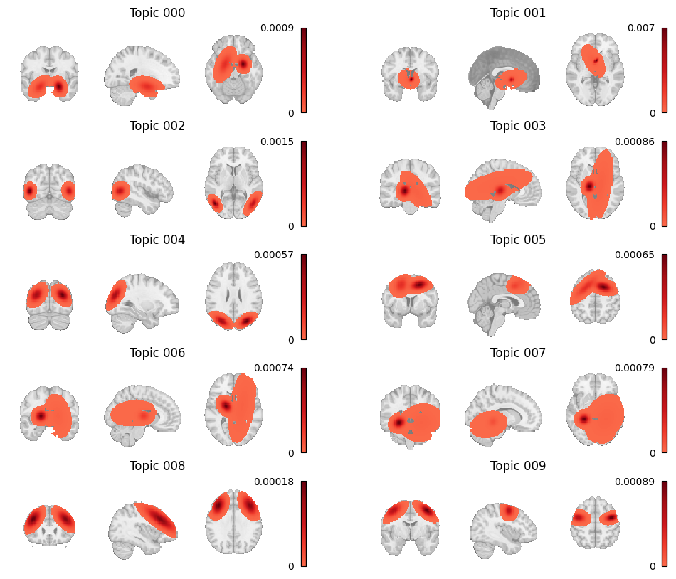
Figure 15:Topic weight maps for the first ten topics in the GCLDA model.
12Meta-Analytic Functional Decoding
Functional decoding performed with meta-analytic data, refers to methods which attempt to predict mental states from neuroimaging data using a large-scale meta-analytic database Smith et al., 2009. Such analyses may also be referred to as “informal reverse inference” Poldrack, 2011, “functional characterization analysis” Bzdok et al., 2013Cieslik et al., 2013Rottschy et al., 2013, “open-ended decoding” Rubin et al., 2017, or simply “functional decoding” Amft et al., 2015Bzdok et al., 2013Nickl-Jockschat et al., 2015. While the terminology is far from standardized, we will refer to this method as meta-analytic functional decoding in order to distinguish it from alternative methods like multivariate decoding and model-based decoding Poldrack, 2011. Meta-analytic functional decoding is often used in conjunction with MACM, meta-analytic clustering, meta-analytic parcellation, and meta-ICA, in order to characterize resulting brain regions, clusters, or components. Meta-analytic functional decoding models have also been extended for the purpose of meta-analytic functional encoding, wherein text is used to generate statistical images Dockès et al., 2018Nunes, 2018Rubin et al., 2017.
Four common approaches are correlation-based decoding, dot-product decoding, weight-sum decoding, and chi-square decoding. We will first discuss continuous decoding methods (i.e., correlation and dot-product), followed by discrete decoding methods (weight-sum and chi-square).
12.1Decoding continuous inputs
When decoding unthresholded statistical maps (such as Figure 16), the most common approaches are to simply correlate the input map with maps from the database, or to compute the dot product between the two maps. In Neurosynth, meta-analyses are performed for each label (i.e., term or topic) in the database and then the input image is correlated with the resulting unthresholded statistical map from each meta-analysis. Performing statistical inference on the resulting correlations is not straightforward, however, as voxels display strong spatial correlations, and the true degrees of freedom are consequently unknown (and likely far smaller than the nominal number of voxels). In order to interpret the results of this decoding approach, users typically select some arbitrary number of top correlation coefficients ahead of time, and use the associated labels to describe the input map. However, such results should be interpreted with great caution.
/srv/conda/envs/notebook/lib/python3.7/site-packages/nilearn/plotting/img_plotting.py:348: FutureWarning: Default resolution of the MNI template will change from 2mm to 1mm in version 0.10.0
  anat_img = load_mni152_template()
/srv/conda/envs/notebook/lib/python3.7/site-packages/nilearn/_utils/niimg.py:62: UserWarning: Non-finite values detected. These values will be replaced with zeros.
  "Non-finite values detected. "
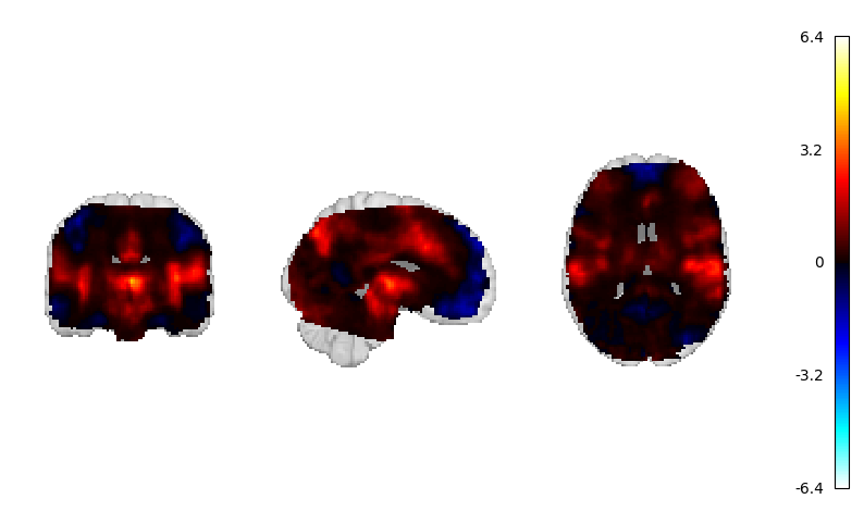
Figure 16:The unthresholded statistical map that will be used for continuous decoding.
This approach can also be applied to an image-based database like NeuroVault, either by correlating input data with meta-analyzed statistical maps, or by deriving distributions of correlation coefficients by grouping statistical maps in the database according to label.
Using these distributions, it is possible to statistically compare labels in order to assess label significance.
NiMARE includes methods for both correlation-based decoding and correlation distribution-based decoding, although the correlation-based decoding is better established and should be preferred over the correlation distribution-based decoding.
As such, we will only show the nimare.decode.continuous.CorrelationDecoder here.
from nimare import decode, meta

corr_decoder = decode.continuous.CorrelationDecoder(
    frequency_threshold=0.001,
    meta_estimator=meta.MKDADensity(kernel_transformer=kern, memory_limit=None),
    target_image="z",
    features=target_features,
    memory_limit="500mb",
)
corr_decoder.fit(neurosynth_dset_first500)
corr_df = corr_decoder.transform(continuous_map)Figure 17:The top ten terms, sorted by absolute correlation coefficient, from the correlation decoding method.
12.2Decoding discrete inputs
Decoding regions of interest (ROIs) requires a different approach than decoding unthresholded statistical maps.
One simple approach, used by GCLDA and implemented in the function nimare.decode.discrete.gclda_decode_roi, simply sums the P(topic|voxel) distribution across all voxels in the ROI in order to produce a value associated with each topic for the ROI.
These weight sum values are arbitrarily scaled and cannot be compared across ROIs.
We will not show this method because of its simplicity and the fact that it can only currently be applied to a GCLDA model.
Before we dig into the other decoding methods are are available, let’s take a look at the ROI we want to decode.
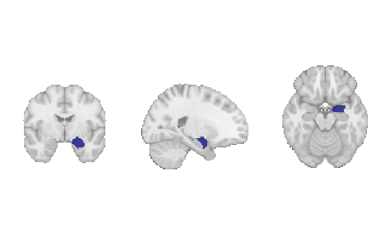
Figure 18:The amygdala region of interest mask that will be used for discrete decoding.
One method which relies on correlations, much like the continuous correlation decoder, is the ROI association decoding method (nimare.decode.discrete.ROIAssociationDecoder), originally implemented in the Neurosynth Python library.
In this method, each study with coordinates in the dataset is convolved with a kernel transformer to produce a modeled activation map.
The resulting modeled activation maps are then masked with a region of interest (i.e., the target of the decoding), and the values are averaged within the ROI.
These averaged modeled activation values are then correlated with the term weights for all labels in the dataset.
This decoding method produces a single correlation coefficient for each of the dataset’s labels.
Figure 19:The top ten terms, sorted by absolute correlation coefficient, from the ROI association decoding method.
A more theoretically driven approach to ROI decoding is to use chi-square-based methods. The two methods which use chi-squared tests are the BrainMap decoding method and an adaptation of Neurosynth’s meta-analysis method.
In both chi-square-based methods, studies are first selected from a coordinate-based database according to some criterion. For example, if decoding a region of interest, users might select studies reporting at least one coordinate within 5 mm of the ROI. Metadata (such as ontological labels) for this subset of studies are then compared to those of the remaining, unselected portion of the database in a confusion matrix. For each label in the ontology, studies are divided into four groups: selected and label-positive (SS+L+), selected and label-negative (SS+L-), unselected and label-positive (SS-L+), and unselected and label-negative (SS-L-). Each method then compares these groups in order to evaluate both consistency and specificity of the relationship between the selection criteria and each label, which are evaluated in terms of both statistical significance and effect size.
12.2.1BrainMap method
The BrainMap discrete decoding method, implemented in nimare.decode.discrete.BrainMapDecoder, compares the distributions of studies with each label within the sample against those in a larger database while accounting for the number of foci from each study.
Broadly speaking, this method assumes that the selection criterion is associated with one peak per study, which means that it is likely only appropriate for selection criteria based around foci, such as regions of interest.
One common analysis, meta-analytic clustering, involves dividing studies within a database into meta-analytic groupings based on the spatial similarity of their modeled activation maps (i.e., study-wise pseudo-statistical maps produced by convolving coordinates with a kernel).
The resulting sets of studies are often functionally decoded in order to build a functional profile associated with each meta-analytic grouping.
While these groupings are defined as subsets of the database, they are not selected based on the location of an individual peak, and so weighting based on the number of foci would be inappropriate.
This decoding method produces four outputs for each label. First, the distribution of studies in the sample with the label are compared to the distributions of other labels within the sample. This consistency analysis produces both a measure of statistical significance (i.e., a p-value) and a measure of effect size (i.e., the likelihood of being selected given the presence of the label). Next, the studies in the sample are compared to the studies in the rest of the database. This specificity analysis produces a p-value and an effect size measure of the posterior probability of having the label given selection into the sample. A detailed algorithm description is presented in .
Figure 20:The top ten terms, sorted by reverse-inference posterior probability, from the BrainMap chi-squared decoding method.
12.2.2Neurosynth method
The implementation of the MKDA Chi-squared meta-analysis method used by Neurosynth is quite similar to BrainMap’s method for decoding, if applied to annotations instead of modeled activation values.
This method, implemented in nimare.decode.discrete.NeurosynthDecoder, compares the distributions of studies with each label within the sample against those in a larger database, but, unlike the BrainMap method, does not take foci into account.
For this reason, the Neurosynth method would likely be more appropriate for selection criteria not based on regions of interest (e.g., for characterizing meta-analytic groupings from a meta-analytic clustering analysis).
However, the Neurosynth method requires user-provided information that BrainMap does not.
Namely, in order to estimate probabilities for the consistency and specificity analyses with Bayes’ Theorem, the Neurosynth method requires a prior probability of a given label.
Typically, a value of 0.5 is used (i.e., the estimated probability that an individual is undergoing a given mental process described by a label, barring any evidence from neuroimaging data, is predicted to be 50%).
This is, admittedly, a poor prediction, which means that probabilities estimated based on this prior are not likely to be accurate, though they may still serve as useful estimates of effect size for the analysis.
Like the BrainMap method, this method produces four outputs for each label. For the consistency analysis, this method produces both a p-value and a conditional probability of selection given the presence of the label and the prior probability of having the label. For the specificity analysis, the Neurosynth method produces both a p-value and a posterior probability of presence of the label given selection and the prior probability of having the label. A detailed algorithm description is presented in .
Figure 21:The top ten terms, sorted by reverse-inference posterior probability, from the Neurosynth chi-squared decoding method.
In both methods, the database acts as an estimate of the underlying distribution of labels in the real world, such that the probability of having a peak in an ROI given the presence of the label might be interpreted as the probability of a brain activating a specific brain region given that the individual is experiencing a given mental state. This is a very poor interpretation, given that any database of neuroimaging results will be skewed more toward the interests of the field than the distribution of mental states or processes experienced by humans, which is why decoding must be interpreted with extreme caution. It is important not to place too much emphasis on the results of functional decoding analyses, although they are very useful in that they can provide a quantitative estimate behind the kinds of interpretations generally included in discussion sections that are normally only backed by informal literature searches or prior knowledge.
The meta-analytic functional decoding methods in NiMARE provide a very rudimentary approach for open-ended decoding (i.e., decoding across a very large range of mental states) that can be used with resources like NeuroVault. However, standard classification methods have also been applied to datasets from NeuroVault (e.g., Varoquaux et al. (2018)), although these methods do not fall under NiMARE’s scope.
13Future Directions
NiMARE’s mission statement encompasses a range of tools that have not yet been implemented in the package. In the future, we plan to incorporate a number of additional methods. Here we briefly describe several of these tools.
13.1Integration with external databases
A resource which may ultimately be integrated with Neurosynth is Brainspell. Brainspell is a port of the Neurosynth database in which users may manually annotate the automatically extracted study information. The goal of Brainspell is to crowdsource annotation through both expert and nonexpert annotators, which would address the primary weaknesses of BrainMap (i.e., slow growth) and Neurosynth (i.e., noise in data extraction and annotation). Annotations in Brainspell may use labels from the Cognitive Paradigm Ontology (CogPO) Turner & Laird, 2012, an ontology adapted from the BrainMap Taxonomy, or from the Cognitive Atlas Poldrack et al., 2011, a collaboratively generated ontology built by contributions from experts across the field of cognitive science. Users may also correct the coordinates extracted by Neurosynth, which may suffer from extraction errors, and may add important metadata like the number of subjects associated with each comparison in each study.
Brainspell has suffered from low growth, which is why its annotations have not been integrated back into Neurosynth, but a new frontend tool for Brainspell, geared toward meta-analysts, has been developed called metaCurious. MetaCurious facilitates neuroimaging meta-analyses by allowing users to iteratively perform literature searches and to annotate rejected articles with reasons for exclusion. In addition to these features, metaCurious users can annotate studies with the same labels and metadata as Brainspell, but with the features geared toward meta-analysts site usage is expected to exceed that of Brainspell proper.
While NiMARE does not natively include tools for interacting with Brainspell or metaCurious, there are plans to support NiMARE-format exports in both services.
13.2Seed-based D-Mapping
Seed-based d-mapping (SDM) Radua et al., 2012, previously known as signed differential mapping, is a relatively recently-developed approach designed to incorporate both peak-specific effect size estimates and unthresholded images, when available. In SDM, foci are convolved with an anisotropic kernel which, unlike the Gaussian and spherical kernels employed in ALE and MKDA, respectively, accounts for tissue type to provide more empirically realistic spatial models of the clusters from the original studies. The SDM algorithm is not yet supported in NiMARE, given the difficulty in implementing an algorithm without access to code.
13.3Model-based CBMA
Model-based algorithms, a recent alternative to kernel-based approaches, model foci from studies as the products of stochastic models sampling some underlying distribution. Some of these methods include the Bayesian hierarchical independent cluster process model (BHICP) Kang et al., 2011, the Bayesian spatially adaptive binary regression model (SBR) Yue et al., 2012, the hierarchical Poisson/Gamma random field model (HPGRF/BHPGM) Kang et al., 2014, the spatial Bayesian latent factor regression model (SBLFRM) Montagna et al., 2018, and the random effects log Gaussian Cox process model (RFX-LGCP) Samartsidis et al., 2019.
Although these methods are much more computationally intensive than kernel-based algorithms, they provide information that kernel-based methods cannot, such as spatial confidence intervals, effect size estimate confidence intervals, and the facilitation of reverse inference. A more thorough description of the relative strengths of model-based algorithms is presented in Samartsidis et al. (2017), but these benefits, at the cost of computational efficiency, have led the authors to recommend kernel-based methods for exploratory analysis and model-based methods for confirmatory analysis.
NiMARE does not currently implement any model-based CBMA algorithms, although there are plans to include at least one in the future.
13.4Additional automated annotation methods
Several papers have used article text to automatically annotate meta-analytic databases with a range of methods. Alhazmi et al. (2018) used a combination of correspondence analysis and clustering to identify subdomains in the cognitive neuroscience literature from Neurosynth text. Monti et al. (2016) generated word and document embeddings in vector space from Neurosynth abstracts using deep Boltzmann machines, which allowed them to cluster words based on semantic similarity or to describe Neurosynth articles in terms of these word clusters. Nunes (2018) used article abstracts from Neurosynth to represent documents as dense vectors as well. These document vectors were then used in conjunction with corresponding coordinates to cluster words into categories, essentially annotating Neurosynth articles according to a new “ontology” based on both abstract text and coordinates.
Meta-analytic databases may also be used in conjunction with existing ontologies in order to redefine mental states or to refine the ontology. For example, Yeo et al. (2016) used the Author-Topic model to identify connections between Paradigm Classes (i.e., tasks) and Behavioral Domains (i.e., mental states) from the BrainMap Taxonomy using the BrainMap database. Other examples include using meta-analytic clustering, combined with functional decoding, to identify groups of terms/labels that co-occur in neuroimaging data, in order to determine if the divisions currently employed in existing ontologies accurately reflect how mental states are separated in the mind (e.g., Laird et al., 2015Riedel et al., 2018Bottenhorn et al., 2019).
14Summary
The advent of open, large-scale databases of neuroimaging results, whether full, unthresholded statistical maps or simple coordinates, has allowed for the development of a wide variety of methods for performing fMRI meta-analyses and related analyses. These methods are often (but not always) released as tools for the community to use, written in a range of languages and with highly variable interfaces. As a consequence, it is difficult for meta-analysts to keep abreast of the current literature and to employ whatever method is most appropriate to address a given question. NiMARE provides a centralized repository for these tools, which will make it easier for researchers to keep track of new methods, and also provides said tools with extensive documentation and a standardized programmatic interface, which will allow researchers to use whatever tool is most appropriate for their research, without unnecessarily steep learning curves.
Given that NiMARE is open source and collaboratively developed on GitHub, methodologists may contribute their own meta-analytic algorithms directly, or interested third parties may implement these algorithms using papers or external tools as a basis for understanding the methods.
15References
16Appendix I: BrainMap Discrete Decoding
The BrainMap discrete decoding method compares the distributions of studies with each label within the sample against those in a larger database while accounting for the number of foci from each study. Broadly speaking, this method assumes that the selection criterion is associated with one peak per study, which means that it is likely only appropriate for selection criteria based around foci, such as regions of interest. One common analysis, meta-analytic clustering, involves dividing studies within a database into meta-analytic groupings based on the spatial similarity of their modeled activation maps (i.e., study-wise pseudo-statistical maps produced by convolving coordinates with a kernel). The resulting sets of studies are often functionally decoded in order to build a functional profile associated with each meta-analytic grouping. While these groupings are defined as subsets of the database, they are not selected based on the location of an individual peak, and so weighting based on the number of foci would be inappropriate.
This decoding method produces four outputs for each label. First, the distribution of studies in the sample with the label are compared to the distributions of other labels within the sample. This consistency analysis produces both a measure of statistical significance (i.e., a p-value) and a measure of effect size (i.e., the likelihood of being selected given the presence of the label). Next, the studies in the sample are compared to the studies in the rest of the database. This specificity analysis produces a p-value and an effect size measure of the posterior probability of having the label given selection into the sample. A detailed algorithm description is presented below.
The BrainMap method for discrete functional decoding performs both forward and reverse inference using an annotated coordinate-based database and a target sample of studies within that database. Unlike the Neurosynth approach, the BrainMap approach incorporates information about the number of foci associated with each study in the database.
Select studies in the database according to some criterion (e.g., having at least one peak in an ROI).
For each label, studies in the database can now be divided into four groups.
Label-positive and selected -->
Label-negative and selected -->
Label-positive and unselected -->
Label-negative and unselected -->
Additionally, the number of foci associated with each of these groups is extracted.
Number of foci from studies with label,
Number of foci from studies without label,
Total number of foci in the database,
Compute the number of times any label is used in the database, (e.g., if every experiment in the database uses two labels, then this number is , where is the total number of experiments in the database).
Compute the probability of being selected, .
, where
For each label, compute the probability of having the label, .
, where
For each label, compute the probability of being selected given presence of the label, .
Can be re-interpreted as the probability of activating the ROI given a mental state.
Convert into the forward inference likelihood, .
Compute the probability of the label given selection, .
Can be re-interpreted as probability of a mental state given activation of the ROI.
This is the reverse inference posterior probability.
Perform a binomial test to determine if the rate at which studies are selected from the set of studies with the label is significantly different from the base probability of studies being selected across the whole database.
The number of successes is , the number of trials is , and the hypothesized probability of success is
If , override the p-value from this test with 1, essentially ignoring this label in the analysis.
Convert p-value to unsigned z-value.
Perform a two-way chi-square test to determine if presence of the label and selection are independent.
If , override the p-value from this test with 1, essentially ignoring this label in the analysis.
Convert p-value to unsigned z-value.
17Appendix II: Neurosynth Discrete Decoding
The implementation of the MKDA Chi-squared meta-analysis method used by Neurosynth is quite similar to BrainMap’s method for decoding, if applied to annotations instead of modeled activation values. This method compares the distributions of studies with each label within the sample against those in a larger database, but, unlike the BrainMap method, does not take foci into account. For this reason, the Neurosynth method would likely be more appropriate for selection criteria not based on regions of interest (e.g., for characterizing meta-analytic groupings from a meta-analytic clustering analysis). However, the Neurosynth method requires user-provided information that BrainMap does not. Namely, in order to estimate probabilities for the consistency and specificity analyses with Bayes’ Theorem, the Neurosynth method requires a prior probability of a given label. Typically, a value of 0.5 is used (i.e., the estimated probability that an individual is undergoing a given mental process described by a label, barring any evidence from neuroimaging data, is predicted to be 50%). This is, admittedly, a poor prediction, which means that probabilities estimated based on this prior are not likely to be accurate, though they may still serve as useful estimates of effect size for the analysis.
Like the BrainMap method, this method produces four outputs for each label. For the consistency analysis, this method produces both a p-value and a conditional probability of selection given the presence of the label and the prior probability of having the label. For the specificity analysis, the Neurosynth method produces both a p-value and a posterior probability of presence of the label given selection and the prior probability of having the label. A detailed algorithm description is presented below.
The Neurosynth method for discrete functional decoding performs both forward and reverse inference using an annotated coordinate-based database and a target sample of studies within that database. Unlike the BrainMap approach, the Neurosynth approach uses an a priori value as the prior probability of any given experiment including a given label.
Select studies in the database according to some criterion (e.g., having at least one peak in an ROI).
For each label, studies in the database can now be divided into four groups:
Label-positive and selected -->
Label-negative and selected -->
Label-positive and unselected -->
Label-negative and unselected -->
Set a prior probability of a given mental state occurring in the real world.
Neurosynth uses
0.5as the default.
Compute :
Probability of being selected, , where and
For each label, compute :
, where and
Compute :
Compute :
Only used to determine sign of reverse inference z-value.
Compute , where is the prior probability of a label:
This is the forward inference posterior probability. Probability of selection given label and given prior probability of label, .
Compute :
This is the reverse inference posterior probability. Probability of label given selection and given the prior probability of label.
Perform a one-way chi-square test to determine if the rate at which studies are selected for a given label is significantly different from the average rate at which studies are selected across labels.
Convert p-value to signed z-value using whether the number of studies selected for the label is greater than or less than the mean number of studies selected across labels to determine the sign.
Perform a two-way chi-square test to determine if presence of the label and selection are independent.
Convert p-value to signed z-value using to determine sign.
18Build Information
nb-exec-table - Unknown Directive
nb-exec-table - Unknown DirectiveAcknowledgments
We would like to thank Yifan Yu and Jérôme Dockès, who provided feedback on the manuscript.
This work was partially funded by the National Institutes of Health (NIH) NIH-NIBIB P41 EB019936 (ReproNim), NIH-NIMH R01 MH083320 (CANDIShare), and NIH RF1 MH120021 (NIDM), the National Institute Of Mental Health under Award Number R01MH096906 (Neurosynth), as well as the Canada First Research Excellence Fund, awarded to McGill University for the Healthy Brains for Healthy Lives initiative and the Brain Canada Foundation with support from Health Canada.
- Pedregosa, F., Varoquaux, G., Gramfort, A., Michel, V., Thirion, B., Grisel, O., Blondel, M., Prettenhofer, P., Weiss, R., Dubourg, V., Vanderplas, J., Passos, A., Cournapeau, D., Brucher, M., Perrot, M., & Duchesnay, E. (2011). Scikit-learn: Machine Learning in Python. Journal of Machine Learning Research, 12, 2825–2830.
- Buitinck, L., Louppe, G., Blondel, M., Pedregosa, F., Mueller, A., Grisel, O., Niculae, V., Prettenhofer, P., Gramfort, A., Grobler, J., Layton, R., VanderPlas, J., Joly, A., Holt, B., & Varoquaux, G. (2013). API design for machine learning software: experiences from the scikit-learn project. ECML PKDD Workshop: Languages for Data Mining and Machine Learning, 108–122.
- Virtanen, P., Gommers, R., Oliphant, T. E., Haberland, M., Reddy, T., Cournapeau, D., Burovski, E., Peterson, P., Weckesser, W., Bright, J., van der Walt, S. J., Brett, M., Wilson, J., Millman, K. J., Mayorov, N., Nelson, A. R. J., Jones, E., Kern, R., Larson, E., … SciPy 1.0 Contributors. (2020). SciPy 1.0: fundamental algorithms for scientific computing in Python. Nat. Methods, 17(3), 261–272.
- Walt, S. van der, van der Walt, S., Chris Colbert, S., & Varoquaux, G. (2011). The NumPy Array: A Structure for Efficient Numerical Computation. In Computing in Science & Engineering (Vol. 13, pp. 22–30).
- Harris, C. R., Millman, K. J., van der Walt, S. J., Gommers, R., Virtanen, P., Cournapeau, D., Wieser, E., Taylor, J., Berg, S., Smith, N. J., Kern, R., Picus, M., Hoyer, S., van Kerkwijk, M. H., Brett, M., Haldane, A., Del Rı́o, J. F., Wiebe, M., Peterson, P., … Oliphant, T. E. (2020). Array programming with NumPy. Nature, 585(7825), 357–362.
- McKinney, W. (2010). Data Structures for Statistical Computing in Python. In Proceedings of the 9th Python in Science Conference.
- Brett, M., Markiewicz, C. J., Hanke, M., Côté, M.-A., Cipollini, B., McCarthy, P., Jarecka, D., Cheng, C. P., Halchenko, Y. O., Cottaar, M., Ghosh, S., Larson, E., Wassermann, D., Gerhard, S., Lee, G. R., Wang, H.-T., Kastman, E., Kaczmarzyk, J., Guidotti, R., … freec84. (2020). nipy/nibabel: 3.1.1 (3.1.1). Zenodo. 10.5281/zenodo.3924343
- Abraham, A., Pedregosa, F., Eickenberg, M., Gervais, P., Mueller, A., Kossaifi, J., Gramfort, A., Thirion, B., & Varoquaux, G. (2014). Machine learning for neuroimaging with scikit-learn. Front. Neuroinform., 8, 14.
- Seabold, S., & Perktold, J. (2010). Statsmodels: Econometric and Statistical Modeling with Python. In Proceedings of the 9th Python in Science Conference.
- da Costa-Luis, C., Larroque, S. K., Altendorf, K., Mary, H., Korobov, M., Yorav-Raphael, N., Ivanov, I., Bargull, M., Rodrigues, N., CHEN, G., Newey, C., James, Zugnoni, M., Pagel, M. D., mjstevens777, Dektyarev, M., Rothberg, A., Alexander, Panteleit, D., … Malmgren, S. (2020). tqdm: A fast, Extensible Progress Bar for Python and CLI (v4.49.0). Zenodo. 10.5281/zenodo.4026750
- Poldrack, R. A., & Yarkoni, T. (2016). From Brain Maps to Cognitive Ontologies: Informatics and the Search for Mental Structure. Annu. Rev. Psychol., 67, 587–612.
- Poldrack, R. A. (2010). Mapping Mental Function to Brain Structure: How Can Cognitive Neuroimaging Succeed? Perspect. Psychol. Sci., 5(6), 753–761.
- Turner, J. A., & Laird, A. R. (2012). The cognitive paradigm ontology: design and application. Neuroinformatics, 10(1), 57–66.
- Fox, P. T., Laird, A. R., Fox, S. P., Fox, P. M., Uecker, A. M., Crank, M., Koenig, S. F., & Lancaster, J. L. (2005). BrainMap taxonomy of experimental design: description and evaluation. Hum. Brain Mapp., 25(1), 185–198.
- Fox, P. T., & Lancaster, J. L. (2002). Opinion: Mapping context and content: the BrainMap model. Nat. Rev. Neurosci., 3(4), 319–321.